Style Transfer
Background
What is Style Transfer?
Style transfer is the technique of recomposing images in the style of other images. For instance, we could take a picture of the Mona Lisa and paint it in a different style:
The Paper:
The idea came about by Leon A. Gatys et al. who plublished A Neural Algorithm of Artistic Style in 2015. They proposed style transfer as an optimization problem which can be solved through training a neural network. Specifically, the authors use a pre-trained convolutional neural network, called the VGG16 model, that has already developed intuition for some internal representation of content and style within a given image.
Prerequisites
Neural Network:
A specific model within the field of deep learning that attempts to mimic how the human brain process information. The neural network moves input data forward through a series layers and calculating weights to create a prediction. The prediction is then compared to the actual value and the network moves backwards to update the weights. The network produces a function $f$ that takes in an input $x$ and produces an output $y$ such that $f(x) = y$.
Convolutional Layers:
Convolution is a mathematical operation that takes a kernel, a fixed square window of weights, and sums the pixel values of the image within the kernel window multiplied by the corresponding kernel weight. Convolution tries to detect the presence of a feature within the kernel window and produces a new window of numbers called a feature map. For example:
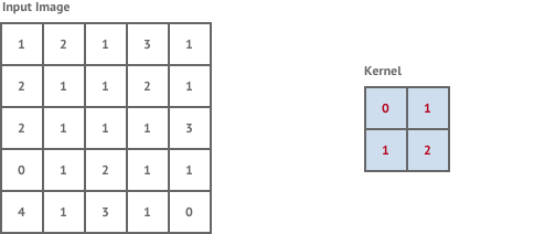
Convolutional layers in neural networks are industry standard for performing tasks such as image classification. The feature maps give us some intuition about what is in the content of an image.
Fully Connected Layers:
A fully connected layer takes an input and multiplies it by a weight matrix and then adds a bias vector.
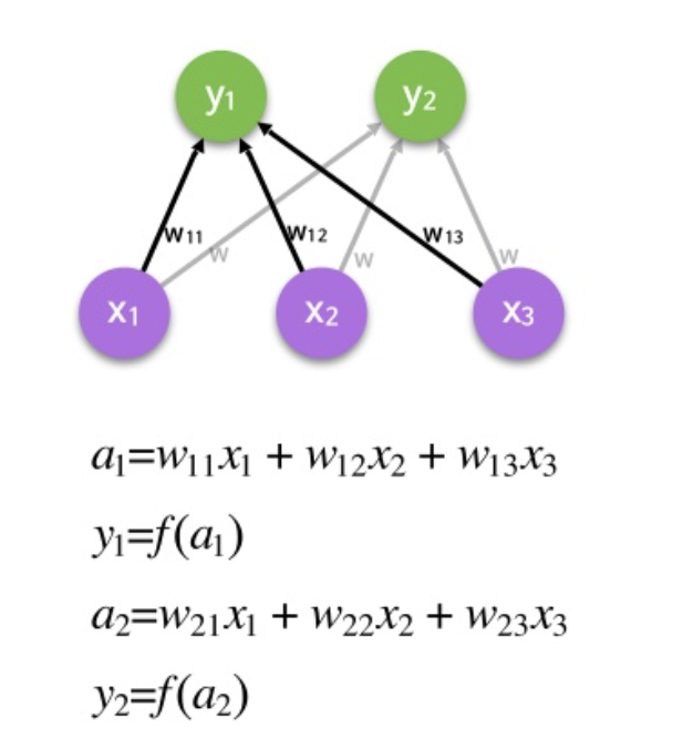
At the end of a convolutional neural network it is common to find a series of fully connected layers. The output in a convolutional layer represents high-level features in the data. Adding a fully connected layer is an easy and cheap way of learning non-linear combinations of these features. Essentially the convolutional layers are providing a meaningful, low-dimensional, and somewhat invariant feature space, and the fully-connected layer is learning a (possibly non-linear) function in that space.
Rectified Linear Units (ReLus):
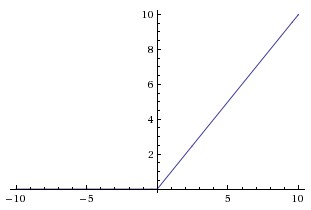
A ReLu is an activation function that computes the function $f(x) = max(0,x)$. The function is quite simple and is frequently used in non-output layers as it speeds up training. The computational step of a ReLu is easy; any negative elements are set to 0.0 and there are no exponentials, no multiplication, and no division operations. ReLu is often computed after the convolution operation and serves as a nonlinear activation function like a hyperbolic tangent (tanh) or sigmoid would be. The ReLu function looks as follows:
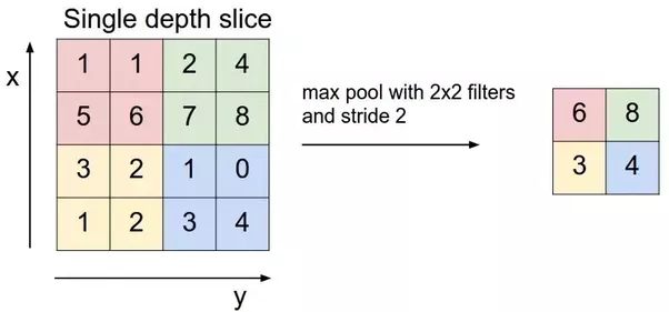
Max Pooling:
Max Pooling is a down-sampling operation on an input representation, it reduces dimensionality and allows for assumptions to be made about features contained in a binned sub-region. The process is as follows:
Max pooling allows some sense of translational invariance. For instance, max pooling allows us to learn that a face has the following components: eyes, nose, lips, and ears. Translational invariance means that as long as these components are present in an image, it does not matter what arangement the components are in. For example:
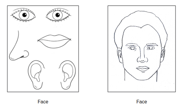
Above, both images would be classified as a face in a network that uses maxpooling as the components for a face are present in both images.
VGG Network:
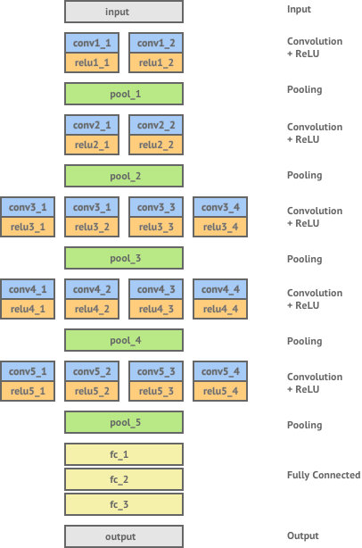
ImageNet is a large scale visual recognition challenge where teams compete to classify millions of images with objects that come from almost 1,000 categories. In 2014, the Visual Geometry Group (VGG) from Oxford University, won this challenge with a classification error rate of only 7.0%. Gatys et. al used this pretrained network for their application of style transfer. The network consists of 16 layers of convolution and ReLU non-linearity, separated by 5 pooling layers and ending in 3 fully connected layers. The architecture is as follows:
Content Representation:
Content is defined as what is in the image. For instance, if we had a picture of the Mona Lisa, the face and body of the painting would be the content. Networks that have been trained for the task of object recognition learn which features it is important to extract from an image in order to identify its content. The feature maps in the convolution layers of the network can be seen as the network's internal representation of the image content. Thus, we can represent the content of an image by extracting the feature map from the convolutional layers in a neural network.
Style Representation:
Style of an image is defined as the way in which the content is presented. For instance, the color and swirly nature in the Starry Night painting represents the style of the paining. The style of an image is not well captured by simply looking at the values of a feature map from the convolutional layer in the neural network. However, Gatys et. al found that we can extract a style representation by looking at the spatial correlation of the values within the feature map. To do this, the Gram matrix of the feature map is calculated. If we have a feature map $F$ represented as a matrix then the Gram matrix $G$ can be calculated with each entry $G_{ij} = \sum_{k}F_{ik}F_{jk}$. Using this, we can see that if we had two images whose feature maps at a given layer produced the same Gram matrix then we would find that the two images had similar style, but not necessairly similar content. Gram et. al found that the best results for style representation came from applying the gram matrix to a combination of shallow and deep layers. Applying this to early layers in the network would capture some of the finer textures contained within the image whereas applying this to deeper layers would capture more higher-level elements of the image’s style.
Optimization:
With style transfer we have the task of generating a new image $Y$, whose style is equal to a style image $S$ and whose content is equal to a content image $C$. Thus, we have to define a loss for our content and style. Let $l$ be a chosen content layer, then the content loss is defined as the euclidean distance between the feature map $F^{l}$ of our content image $C$ and the feature map $P^{l}$ of our generated image $Y$. We define the content loss $$L_{\text{content}} = \frac{1}{2}\sum_{ij}\left(F_{ij}^l - P_{ij}^l\right)^2$$. For a chosen style layer $l$, the style loss is defined as the euclidean distance between the Gram matrix $G^l$ of the feature map of our style image $S$ and the Gram matrix $A^l$ of the feature map of our generated image $Y$. We define the style loss $$L_{\text{style}} = \frac{1}{2}\sum_{l=0}^L\left(G_{ij}^l - A_{ij}^l\right)^2.$$ We can now take a weighted sum of the style and content losses, where we can adjust weights to preserve more of the style or more of the content. The total loss $$l_{\text{total}} = \alpha L_{\text{content}} + \beta L_{\text{style}}$$ where $\alpha, \beta \in \mathbb{R}$.We now can perform the task of style transfer by trying to generate an image $Y$ which can minimize the loss function $L_{\text{total}}$.
The Full Pipeline:
The pipeline of the style transfer can be depicted visually as follows:
Above we use forward and backward propogation to minimize our loss.
Code
#Imports

#Data Handling
import numpy as np

#Image Handling
from PIL import Image

#Plotting
import matplotlib.pyplot as plt

#Deep Learning
from keras import backend as K
from keras.applications import vgg16
from keras.applications.vgg16 import preprocess_input
from keras.preprocessing.image import load_img, img_to_array
from keras.applications import VGG16

#Optimization
from scipy.optimize import fmin_l_bfgs_b
Step 1: Load and Preprocess Images
The first step is to load the content and style images and preprocess them.
def preprocessImage(content_image,style_image,targetHeight,targetWidth):
    target_shape = (targetHeight,targetWidth)

    #Load the content image
    cImage = load_img(path=content_image,target_size=target_shape)
    cImageArr = img_to_array(cImage)
    cImageArr = K.variable(preprocess_input(np.expand_dims(cImageArr,axis=0)), dtype="float32")

    #Load the style image
    sImage = load_img(path=style_image,target_size=target_shape)
    sImageArr = img_to_array(cImage)
    sImageArr = K.variable(preprocess_input(np.expand_dims(sImageArr,axis=0)), dtype="float32")

    #Generate some noise
    gImage = np.random.randint(256, size=(targetWidth, targetHeight, 3)).astype('float64')
    gImage = preprocess_input(np.expand_dims(gImage, axis=0))
    gImagePlaceholder = K.placeholder(shape=(1, targetWidth, targetHeight, 3))

    return cImageArr, sImageArr, gImage, gImagePlaceholder
Step 2: Get the Feature Representation:
Here we get the feature representation for an input $x$ for one or more layers in our model.
def getFeatureRepresentation(x,layer_names,model):
    featMatrices = []
    for ln in layer_names:
        selectedLayer = model.get_layer(ln)
        featRaw = selectedLayer.output
        featRawShape = K.shape(featRaw).eval(session=tf_session)
        N_l = featRawShape[-1]
        M_l = featRawShape[1]*featRawShape[2]
        featMatrix = K.reshape(featRaw, (M_l, N_l))
        featMatrix = K.transpose(featMatrix)
        featMatrices.append(featMatrix)
    return featMatrices
Step 3: Get the Content Loss:
We need to return the content loss $$L_{\text{content}} = \frac{1}{2}\sum_{ij}\left(F_{ij}^l - P_{ij}^l\right)^2$$.
def getContentLoss(F, P):
    L_content = 0.5*K.sum(K.square(F - P))
    return L_content
Step 4: Get the Gram Matrix:
We need to calculate the Gram matrix for our style.
def getGramMatrix(F):
    gram_matrix = K.dot(F,K.transpose(F))
    return gram_matrix
Step 5: Get the Style Loss:
We need to return the style loss $$L_{\text{style}} = \frac{1}{2}\sum_{l=0}^L\left(G_{ij}^l - A_{ij}^l\right)^2$$
def getStyleLoss(ws, Gs, As):
    sLoss = K.variable(0.)
    for w, G, A in zip(ws, Gs, As):
        M_l = K.int_shape(G)[1]
        N_l = K.int_shape(G)[0]
        G_gram = getGramMatrix(G)
        A_gram = getGramMatrix(A)
        sLoss+= w*0.25*K.sum(K.square(G_gram - A_gram))/ (N_l**2 * M_l**2)
    return sLoss
Step 6: Get the total loss:
We need to return the total loss as $$l_{\text{total}} = \alpha L_{\text{content}} + \beta L_{\text{style}}$$
def getTotalLoss(gImagePlaceholder,alpha=1.0,beta=1000.0):
    F = getFeatureRepresentation(gImagePlaceholder, layer_names=[cLayerName], model=gModel)[0]
    Gs = getFeatureRepresentation(gImagePlaceholder, layer_names=sLayerNames, model=gModel)
    contentLoss = getContentLoss(F, P)
    styleLoss = getStyleLoss(ws, Gs, As)
    l_total = alpha*contentLoss + beta*styleLoss
    return l_total
Step 7: Minimization of Loss:
Calculate total loss from our generated image to minimize the loss function.
def calculate_loss(gImArr):
    if gImArr.shape != (1, targetWidth, targetWidth, 3):
        gImArr = gImArr.reshape((1, targetWidth, targetHeight, 3))
    loss_fcn = K.function([gModel.input], [getTotalLoss(gModel.input)])
    return loss_fcn([gImArr])[0].astype('float64')
Step 8: Calculate Gradient of Loss:
Calcualte the gradient of the loss function with respect to the generated image.
def get_grad(gImArr):
    if gImArr.shape != (1, targetWidth, targetHeight, 3):
        gImArr = gImArr.reshape((1, targetWidth, targetHeight, 3))
    grad_fcn = K.function([gModel.input],
                          K.gradients(getTotalLoss(gModel.input), [gModel.input]))
    grad = grad_fcn([gImArr])[0].flatten().astype('float64')
    return grad
Step 9: Instantiate Model:
#The Content Image
print("Content Image: ")
plt.imshow(Image.open("content_images/eiffel_tower.jpg"))
plt.show()
#The Style Image
print("\nStyle Image:")
plt.imshow(Image.open("style_images/starry_night_van_goh.jpg"))
plt.show()


#Paths for content and style images
content_image_path = "content_images/eiffel_tower.jpg"
style_image_path = "style_images/starry_night_van_goh.jpg"

#Content Image Properties
cImageOrig = Image.open(content_image_path)
cImageSizeOrig = cImageOrig.size

#Path for output image
genImOutputPath = "results/eiffel_tower_starry_night.jpg"

#Target height/width for images
targetHeight = 512
targetWidth = 512
cImageArr, sImageArr, gImage, gImPlaceholder = preprocessImage(content_image_path,
                                            style_image_path,targetHeight,targetWidth)


#Setup Session
tf_session = K.get_session()

#Select Models
cModel = VGG16(include_top=False, weights='imagenet', input_tensor=cImageArr)
sModel = VGG16(include_top=False, weights='imagenet', input_tensor=sImageArr)
gModel = VGG16(include_top=False, weights='imagenet', input_tensor=gImPlaceholder)

#Select layers for content and style
cLayerName = 'block4_conv2'
sLayerNames = [
                'block1_conv1',
                'block2_conv1',
                'block3_conv1',
                'block4_conv1',
                ]

#Get initial feature representations
P = getFeatureRepresentation(x=cImageArr, layer_names=[cLayerName], model=cModel)
P = P[0]
As = getFeatureRepresentation(x=sImageArr,layer_names=sLayerNames,model=sModel)
ws = np.ones(len(sLayerNames))/float(len(sLayerNames))

#Number of training epochs
iterations = 500

#Minimize the loss using the L-BFGS-B algorithm
x_val = gImage.flatten()
xopt, f_val, info= fmin_l_bfgs_b(calculate_loss, x_val, fprime=get_grad,
                            maxiter=iterations, disp=True)
Step 10: View Results:
def postprocess_array(x):
    # Zero-center by mean pixel
    if x.shape != (targetWidth, targetHeight, 3):
        x = x.reshape((targetWidth, targetHeight, 3))
    x[..., 0] += 103.939
    x[..., 1] += 116.779
    x[..., 2] += 123.68
    # 'BGR'->'RGB'
    x = x[..., ::-1]
    x = np.clip(x, 0, 255)
    x = x.astype('uint8')
    return x

def reprocess_array(x):
    x = np.expand_dims(x.astype('float64'), axis=0)
    x = preprocess_input(x)
    return x

def save_original_size(x, target_size=cImageSizeOrig):
    xIm = Image.fromarray(x)
    xIm = xIm.resize(target_size)
    xIm.save(genImOutputPath)
    return xIm


xOut = postprocess_array(xopt)
xIm = save_original_size(xOut)
#View Generated Image
#Result
print("Style Transfer Image:")
plt.imshow(Image.open("results/eiffel_tower_starry_night.jpg"))
plt.show()

The Training Process:
Tips:
- Different Weightings: Try setting $\alpha$ and $\beta$ to different values. Typically we want $\frac{\beta}{\alpha} \sim 10^5$
- More Style Layers: Add more style layers into sLayerNames, this will be computationally more expensive though.
- More Content Layers: Try adding more content layers.
- Different Model Architectures: Try using different architectures like VGG19, ResNet, or Inception instead of VGG16.
Bonus:
The Neural Style Transfer model uses the VGG16 architecture. This architecture can be built in keras as follows:
#Imports
from keras.models import port Sequential
from keras.layers import Input, Dense, Flatten, Conv2D, MaxPooling2D
from keras.optimizers import SGD
#Define an input shape
inpt_shpe = (150,150,3)
output_dim = 10

#Define the number of classes to output in the multi-class classification problem
def VGG16(inpt_shpe,output_dim):

    #Initialize Model
    model = Sequential()
    #model.add(InputLayer(input_shape=inpt_shpe))
    model.add(Input(input_shape=inpt_shpe))

    #Block 1
    model.add(Conv2D(64, (3, 3), activation='relu', padding='same'))
    model.add(Conv2D(64, (3, 3), activation='relu', padding='same'))
    model.add(MaxPooling2D((2, 2), strides=(2, 2)))

    #Block 2
    model.add(Conv2D(128, (3, 3), activation='relu', padding='same'))
    model.add(Conv2D(128, (3, 3), activation='relu', padding='same'))
    model.add(MaxPooling2D((2, 2), strides=(2, 2)))

    #Block 3
    model.add(Conv2D(256, (3, 3), activation='relu', padding='same'))
    model.add(Conv2D(256, (3, 3), activation='relu', padding='same'))
    model.add(Conv2D(256, (3, 3), activation='relu', padding='same'))
    model.add(MaxPooling2D((2, 2), strides=(2, 2)))

    #Block 4
    model.add(Conv2D(512, (3, 3), activation='relu', padding='same'))
    model.add(Conv2D(512, (3, 3), activation='relu', padding='same'))
    model.add(Conv2D(512, (3, 3), activation='relu', padding='same'))
    model.add(MaxPooling2D((2, 2), strides=(2, 2)))

    #Block 5
    model.add(Conv2D(512, (3, 3), activation='relu', padding='same', name='block5_conv1'))
    model.add(Conv2D(512, (3, 3), activation='relu', padding='same', name='block5_conv2'))
    model.add(Conv2D(512, (3, 3), activation='relu', padding='same', name='block5_conv3'))
    model.add(MaxPooling2D((2, 2), strides=(2, 2), name='block5_maxpool'))

    #Classification Block
    model.add(Flatten(name='flatten'))
    model.add(Dense(4096,activation='relu',name='fc1'))
    model.add(Dense(4096,activation='relu',name='fc2'))
    model.add(Dense(output_dim,activation='softmax',name='predictions'))

    #Compile model with stochastic gradient descent optimizer
    sgd = SGD(lr=0.1, decay=1e-6, momentum=0.9, nesterov=True)
    model.compile(optimizer=sgd,loss='categorical_crossentropy')

    return model